Tech Talk

The on-axis curve is self-explanatory – it is an on-axis measurement.  We can see that it isn’t ruler flat in this anechoic measurement – there are small peaks and dips throughout.  But they aren’t audible because the area under the curve in the region of the deviation is so similar to that of the surrounding area.  The dip at about 11.5 kHz is so narrow that it still preserves most of the area in its little region of the curve.  In fact, when this speaker is measured in a listening room, it measures flat.

The listening window is simply an average over a small window (+/- 10° vertically, axial, and +/- 10°, 20°, and 30° horizontally).  This gives an idea of the average character of the speaker in the most common region a prime listener experiences the speaker from.  It is smoother due to averaging the multiple curves.

The curve for first reflections is where it starts to get interesting.  This is a weighted average of energy in 10° increments from 30° to 70°.  The heaviest weighting is at the angles most common for speakers and listening positions in common rooms that are used for speakers by end-users.  This is the curve that will show how impactful the reflection of highest energy – the first reflection – will be on the speaker’s performance.  We can see for this speaker it is … somewhat boring.  It drops away in level, causing it to have little influence.  It has few deviations from smooth to call attention to itself, and further – what deviations it has are slow trends and nothing sudden.  So it won’t negatively affect the performance.

The soundpower curve is similar to the first reflection curve but adds in all of the rest of the measurements that we take around the speaker using weighting based on area of the sphere for the angle.  But the same expectations and observations can be made as for the first reflection curve.

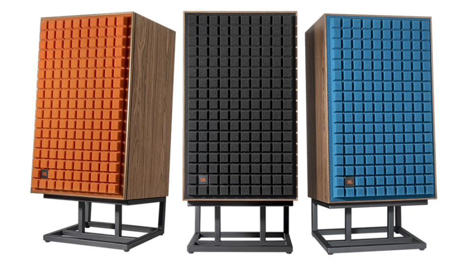
The DI (directivity index) curves are a little different, but easy to understand.  They are the difference amount resulting from subtracting the associated measurement (such as the first reflection curve) from the axial curve.  This is an agreed-upon standard in our industry to characterize the directionality of a sound source.  You can see that these curves climb with frequency, as you would expect since high frequencies are more directional than low frequencies.  In these measurements, due to involvement of vertical angles, there is a lack of smoothness in the 500 to 900 Hz region.  But it is very difficult to get very much off-axis vertically with this speaker (the JBL Synthesis SCL-1), so this isn’t a fair representation of the actual experience.  But we follow the standard measurement.

(Thank you to the JBL Synthesis SCL-1 for the loan of its anechoic-equalized spin curve!)

Discussion

I understand that all of that may have been a bit much.  “Too technical!”, I hear the screams.  But the main thing to take away is that in looking at this measurement as we develop a speaker system, we can work toward a smooth measurement with transitions more like trends than sudden jerks, and peaks and dips are very narrow with little energy difference to keep them difficult if not impossible to hear.  And this keeps the reflected energy from the room benign and allows the speaker to sound great in many different rooms, rather than sounding good in one room and bad in another.  Also, note that as you look higher in frequency response or directivity, you see indications of the level going down – as if you are off-axis on a directional transducer.  This last will help with how a system engineer works with design after Dr. Toole’s discovery.

So, although we can’t compensate for every room, we CAN control the speaker’s “stray” energy to make the “room sound” have much less effect on the performance.

But how smooth does the response have to be?  Since a speakers’ output is a complex sum of a pistonic diaphragm (at some frequencies) with breakup and resonances at most others, no speaker measures flat like an amplifier.  Fortunately, the ear doesn’t hear like our test equipment for amplifiers and does not have infinite resolution.

I didn’t find any papers on this, but I did bring it up with Dr. Olive once.  He said that the ear works like a smoothed measurement and the smoothing was somewhere between 1/3 octave and 1/6 octave.  Since you can notice areas raised above or depressed below others, there is likely a “tracking filter” function, but this is likely due to the fact that the brain, with a memory and rating system is attached to the “measurement.”  In other words, the ear is the SPL meter, and the brain the analyzer and memory as well as imagination to piece together a frequency response.

But this does mean that the ear picks up on relative level of frequency bands, but not small, narrow peaks that are minimized by the smoothing.  The ear can hear a 1 dB difference, but it will be from a mainly flat speaker to an area that could be quite large – 1/3 octave or greater – without listening training.  As a raised (or depressed) area of the response gets narrower, it is more difficult for the ear to pick up on it even with listening training.  For instance, a 2 dB peak or dip at 8 kHz that is 500 to 800 Hz wide will likely not be heard.  From this, it is likely that the ear hears the difference in the area under the curve in two smoothed regions rather than the peaks or dips the eye sees in the graph.

Clearly a good topic to study, but as a system engineer, I wouldn’t know where to start.  Most of what I mentioned in the last paragraph comes from knowing the frequency response of speakers that I have designed and discussing with listeners what they heard. 

So, what does this mean for system design?  Has it made changes in design methods?  And what benefits has it brought to the end-user?

There are some interesting points to consider while designing:

• Some peaks/dips telegraph that they can be removed. If a peak or dip exists in all curves of a spin, it can be filtered or equalized out.  If it exists in only one, the axial curve for example, then the off-axis averages will be damaged when the axial curve is corrected.  This helps with knowing what deviations to go after passively, or what features a “system in a box” must include for good audio reproduction.

• You want the soundpower to roll off. Except for the special case of a true omni-directional speaker, if the soundpower measurement was flat, then the axial measurement would climb as frequency went higher above about 1 – 2 kHz.  This would make for a very bright and harsh speaker system.  Designing for a flat axial and letting the soundpower roll off further helps minimize the reflected level where our ears are the most sensitive – higher frequencies.

• It is even more important to get driver selection correct. The higher frequency driver (midbass, midrange, or tweeter) of a pairing with a lower frequency driver (woofer, midbass, or midrange) must go down low enough in frequency so that it crosses over to the lower frequency driver of the pairing where it has reasonable or matching dispersion.  If it doesn’t, there will be a dip in the soundpower and it will be noticed.  In a multi-way system, the higher-frequency drivers must be able to get down to the frequency of beaming of the next transducer down at higher level than that transducer and handle enough power to keep up with that transducer.

• It is even better if the higher frequency driver of a pairing has a natural dispersion that matches, or its dispersion can be shaped to match, that of the lower frequency driver at the intended crossover frequency. When the pattern of the lower frequency driver matches that of the higher frequency driver at crossover, it is very easy to have a smooth soundpower for the system.
  1. This is why we use waveguides and horns so much, and also why they are near the size of the lower frequency driver. Both drivers and waveguides are ruled by the “the larger it is, the more directional it is at higher frequencies” rule of physics.  And waveguides and horns help control dispersion.

• Coupling point 2 with sensitivity – the high frequency driver must always be more sensitive than the low frequency driver – along with keeping the resonance of the higher frequency driver below the intended crossover frequency points toward more robust high frequency transducers. It is not possible to create smooth soundpower speakers with inexpensive high frequency transducers.

• Lastly, usual rules of thumb – placing transducers that crossover to each other as close together as possible, making sure that the system curve is a positive summation of the transducers, and the like become even more critical. As you make a smooth response, whether it is axial or soundpower, smaller deviations created by cutting corners can be noticed much more easily.

There are many challenges to designing and building a reliable speaker system with good axial and soundpower measurements.  You may ask “Then why do you do it?”

The most important reason was previously mentioned.  The room is made up typically of hard reflectors and reflectors with absorbers on them.  The reflecting surface makes very little change to the character of the sound, whereas a thin absorber will absorb high frequencies but allow the underlying reflective surface to reflect low frequencies.  When the soundpower measurement shows us that off-axis energy forms a smooth curve, then the energy reflected from both to the listener in the room blends positively with the speaker output.  The downward slope to high frequencies also helps minimize the effect of the reflections where our ears are most acute.

This affords the speaker the characteristic that it sounds the same way in any room.  When a speaker works like this, fewer of them are returned to the retailer because it sounds the same at home as at the dealer and more people have good comments in their online speaker reviews.

One would think that would already be a great reason to do this, but it goes further.  This is because when you add a smooth, rolled-off-at-HF version of the speaker’s axial response back with the speaker, the minor delay of normal rooms doesn’t hurt the time domain, or phase, response of the speaker.  When the speaker’s time response is kept intact, then the speaker’s imaging is no longer about left placement, center mono image, and right image.  It suddenly becomes an image that extends to left and right beyond the speakers.  Voices sound so coherent that it seems like the person is in the room with you.  Electronic music that gets away with playing with phase can throw sounds through you and behind you.  I have even run into recordings that image vertically, like the sound of fire running up the back and side walls.

When the speaker images to this degree, it does not take long for the tie of the music to the speaker to break down.  The music becomes a separate thing in the room from the speakers, that now look like simple objects and not sound creation devices.  And reproduced music feels like a special concert for an audience of one.

And that is the reason to jump through the hoops, design legendary transducers, indulge the crossover component manufacturers’ wildest dreams, and to chase the idea of a smooth soundpower measurement:  So that those looking for joy in their music can find it, and they can also rediscover old associated memories.