Tech Talk

By Dylan Constan-Wahl, Principal Engineer

Whenever we listen to a music recording, we also inherently hear the characteristics of the recording and playback process. Analog recording processes were well known by their particular qualities and limitations, whether it was Edison’s wax cylinders, cassette tapes or vinyl LPs. Many of us have experienced the effects of tape hiss, wow and flutter, tracking distortion, and rumble.

Early digital audio processes also exhibited plainly audible limitations like significant transport jitter and error rates. CD audio also had a limited bit depth (16 bits) and a low sample rate (44.1kHz) which meant that the reconstruction filter was extremely difficult to design in an optimal way.

We now live in a remarkable period where the digital audio recording/playback process has the potential to record/reproduce the highest audio dynamic range and timing resolution ever possible. Bit depths up to 32 bits (or floating-point representations beyond this), sample rates up to 768kHz, DSD audio at multiples of the original clock rate are now readily achievable. Modern digital audio presents music artists and listeners with a remarkable medium, on which every musical intention of the artist can be communicated to the listener as if they were present at the recording studio.

At the same time, these high bit depths and sample rates have meant that every element of a piece of audio equipment must be re-evaluated and optimized. Digital to analog conversion, at its heart, means the reproduction of a precise signal level at exactly the correct relative moment in time. Errors in timing and errors in level both show up in the reproduced signal as either noise, harmonic distortion or non-harmonic signal-related distortion.

Reference Clock
The heart of a high-quality digital-to-analog converter is the reference clock. A stable, low noise clock ensures that the DAC chip has a fighting chance of converting samples to the analog domain at precise intervals, ensuring highest fidelity to the recording. In addition, any processes (asynchronous sample rate conversion, oversampling, buffering) designed to filter incoming data jitter depend on the purity of this clock.
How do we characterize the quality of a reference clock? We must first recognize that we can analyze the reference clock both in the time domain and in the frequency domain.

Jitter
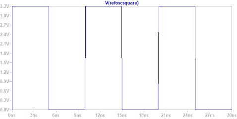
In the time domain, imperfections in the reference clock are measured as timing differences between each cycle of this clock and an idealized clock. For purposes of time domain analysis, we can assume the reference clock is a square wave, as shown in figure 1.

We can measure jitter as:
• the total timing error over an interval,
• the error in the length of each cycle of our reference clock,
• or the difference in time between any two adjacent clock periods.

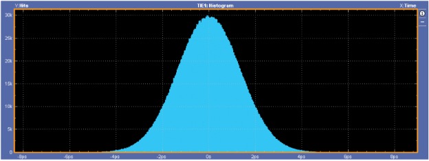
Typically, we use an oscilloscope, which plots signal level versus time, and we capture thousands of clock periods, timed against a near-ideal clock, and plot statistics on the timing error of our reference clock as a histogram, where the mean clock period is in the center of the histogram. The shape of this histogram can hint to us as to whether the jitter present is being generated by a random or non-random process, based on the shape of the histogram. Figure 2 is an example of a histogram of a random jitter from a reference clock.

Phase Noise
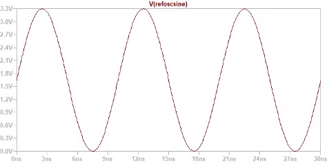
Another way to look at reference clock imperfections is in the frequency domain, or a plot of signal level versus frequency. Whether the reference clock output is in fact a sine wave or a square wave, we are most interested in the fundamental frequency. For simplicity, let’s assume that the reference clock output is a sine wave. An ideal spectrum of a noiseless sine wave clock is shown in figure 3.

When a clock has jitter in the time domain (variation in its period), in the frequency domain this shows up as phase noise. Phase noise is variation in the phase of a clock signal at some rate(s) determined by the type of noise present.

The frequency spectrum plot of a sine wave with phase noise is symmetrical around the fundamental frequency of the clock, as shown in figure 4.

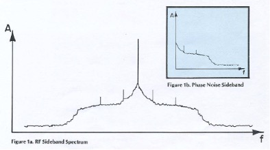
Frequencies below the fundamental are considered as the lower sideband, frequencies above the fundamental are the upper sideband. We typically look at the spectrum of the upper sideband alone, as it’s easier to understand (the frequencies increase from left to right on the x-axis).

This phase noise plot is extremely helpful for an electrical engineer. In the time domain, we only know the total amount of jitter present and a histogram that hints at whether the jittering process is random or not. The phase noise frequency plot identifies the noise in the modulation of our reference clock at each frequency, allowing us to hunt out root causes. For example, a spike of noise at a specific frequency may occur due to interference with the harmonic of another clock or data line in the system. Low frequency phase noise (random walk FM) is typically due to mechanical vibration or temperature variation. Figure 5 outlines the phase modulation frequency ranges associated with different types of noise source in a clock oscillator.

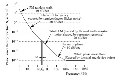
This is helpful in determining what is causing a particular phase error.

How does this all work out in practice? I was evaluating the performance of two different reference clock oscillators for use with a digital-to-analog converter circuit. Both had a fundamental frequency of around 75MHz, and the time domain jitter measurements were within 20%. When I tried locking to some higher bit rate audio using this new oscillator, I experienced audio dropouts and unusual sounding distortion.

To investigate, I used a spectrum analyzer with a high impedance active differential probe to observe the phase noise of my previous reference clock and this new clock under test. Figure 6 shows a phase noise plot of the new reference clock under evaluation, and figure 7 shows the phase noise of the previous reference clock.

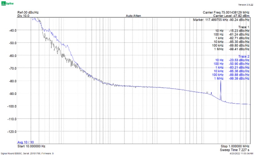
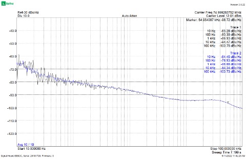
The blue plot in the figures represents an average of 10 phase noise measurements, the black trace is the last phase noise measurement.

As you can see, the evaluated clock had much higher random walk FM phase noise and semiconductor flicker noise than my original reference.

Conclusion
Modern, high bit rate, high sample rate digital audio formats allow us to hear music recordings with an astounding level of fidelity, but also present unique technical challenges for the designers of audio hardware.

By paying close attention to reference clock jitter and phase noise, we can hear closer to the artist’s intended performance than ever before.