Tech Talk

I have worked as an electronic engineer for over 20 years and have designed dozens of different products and hundreds of PCBs in that time. No matter how simple or complex the product or PCB, the one common thing they all share is once that first prototype lands on the work bench, I need to make sure it works as expected. In my experience there are three tools that will be involved in the process of getting the thing to work, or more likely, finding out why it doesn’t work!

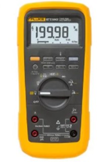
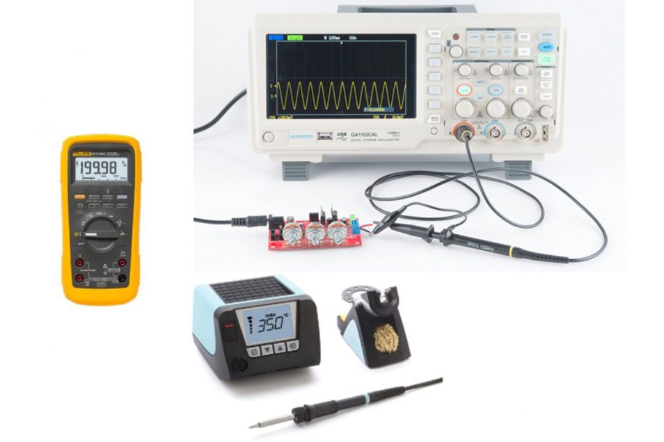
First up, the Swiss army knife of electronic engineering, the Digital Multimeter (DMM).

As the name suggests, the Multimeter performs several functions, but the main use cases are continuity checks, voltage measurement and current measurement.

Continuity checks are the first thing to check on any new PCB before any thoughts of applying power are entertained. Are there any short circuits between the power rails and ground? Are parts of the circuit connected as expected? I have lost count of the number of times a small amount of solder has shorted out rails or internal cables have not been connected correctly, both of which would have resulted in at best the device not turning on and at worst a big bang and lots of smoke resulting in an embarrassing conversation with your boss about why you need a new expensive prototype. Five minutes with a continuity checker is time and money well spent.

Once you have ascertained that the power rails are not shorted out and are connected correctly, the time comes to apply some power to the thing. As soon as power is applied, all the power rails need to be checked to make sure they are all within the expected voltage range. A quick check here to make sure any variable output voltage regulators have been set correctly for example is time well spent.

Measuring the current a particular component or product is drawing typically gets done when something is getting much hotter than expected, which is generally the sign that something isn’t behaving correctly. A simple check with the DMM and a check against the relevant datasheet will ascertain if something is wrong with the power supply or the part of the circuit it is powering.

Once we have got to the stage that the product has power applied and there have been no smoke signals or fireworks, we need to check if the circuit is working as we expect. Typically in electronic design there will be several silicon integrated chips (ICs) on the PCB, all of which will relate to control, data or clock signals. Some of these signals will be simple “always on” or “always off”, in which case your DMM can easily show you if the voltage is present or not - on or off in other words. However, the signals that allow the IC to perform its assigned task are typically switching between on and off incredibly quickly. Switching frequencies of 50MHz (50 million times a second!) are commonplace when dealing with digital audio. How can we measure this easily to ascertain if the frequency is what we expect and if its voltage level is what we expect? The DMM is no use here as its measurement time is probably measured in half-second intervals. Time to break out the oscilloscope.

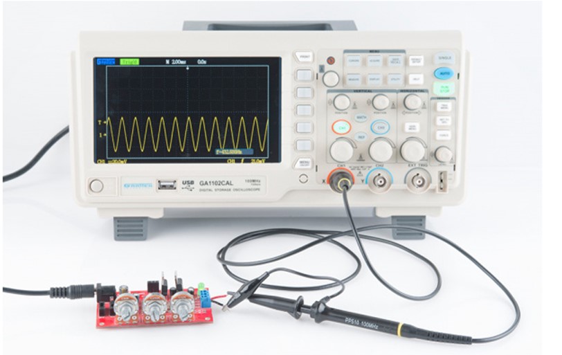
My first experience of an oscilloscope (more commonly referred to as a scope) was more of a panicked “What on earth do all these buttons and knobs do?” sort of affair, but while the scope looks complicated, in most cases it’s very easy to use and incredibly useful. Once the measurement probe is connected to the signal or point of interest on the circuit, the scope shows you the voltage variations of the signal and when these variations are occurring by drawing it on screen. This graphical representation of the signal is referred to as a trace. The level is represented by the height of the trace on screen, the speed at which the signal is changing is represented by the width of the traces on screen.

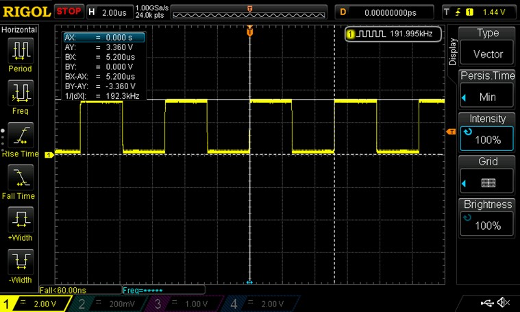
The picture above is a capture of an audio clock. The clock itself is represented by the yellow trace. The grid in the background gives us the voltage and time scales. In this example every vertical grid line represents two volts, so we can see our voltage is between 2 and 4 volts.

Every horizontal grid line represents a unit of time; in this example every line represents 2 microseconds (uS) so we can see for the signal to go from high to low and back to high again takes about 5uS, which works out to be 200kHz.

Helpfully, scopes have cursors you can line up with the edges so you can accurately measure the voltage and time (and therefore frequency) of a signal. As shown on the example above the voltage is actually 3.3V and the frequency is actually 192kHz, which as it happens is the sample rate for the digital audio clock being measured.

The amount of voltage and time for each gridline is variable, which allows the scope to represent very large or very small voltages or units of time in a way where it can be seen on screen. For example, in the screen above if the voltage was above 8 volts, then it would go off the screen, so to measure a voltage above 8 volts, we would change the voltage scale to 5 volts per grid line.

If the signal was faster, we can change the horizontal grid to represent a smaller unit of time (what is known as changing the time base).

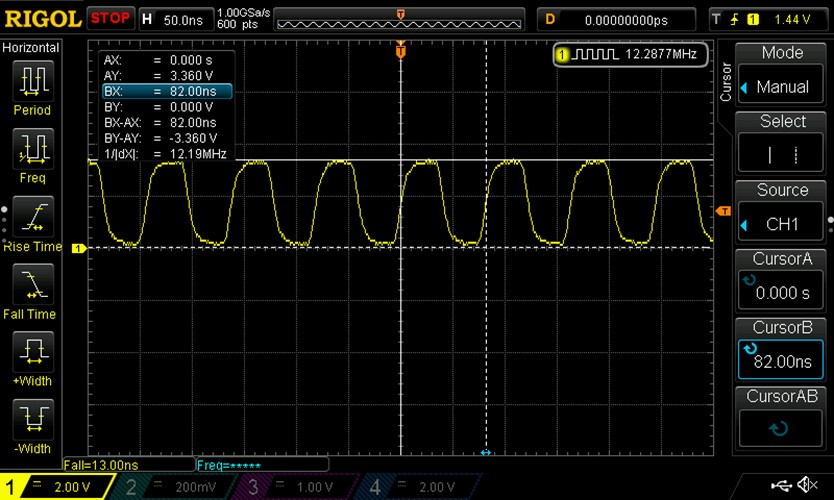
In the example below we are measuring a clock that is the same voltage level but is significantly faster, so in this case we change the time base to be 50 nano seconds (nS) per grid line. Now we can see the clock properly and measure its frequency, which is 12.19Mhz.

Scopes have at least two inputs (or channels). The useful thing here is the scope can show us what a signal looks like with respect to another signal. This is incredibly useful when looking at when a data line is changing with respect to its clock or to check the order in which voltage rails might switch on and how long it takes. These features alone make the scope an invaluable tool in any debug task, and for measurements that are all but impossible to do without a scope.

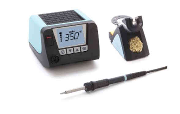
Now the DMM and scope can tell you if something is working but inevitably at some point in the process something won’t be working as expected and something will need to be fixed or modified on the circuit board. Time to warm up the soldering iron.

Something that all circuit boards share is how the parts are physically attached to them, the parts are all soldered. Soldering is a process that uses a molten tin and silver alloy to join the pins or pads of an electronic part to the copper, silver or gold pad of the PCB. Once the solder cools it forms what can be assumed to be a permanent joint between component and PCB.

The soldering iron is a very simple tool at heart. One end - the one that goes in your hand - is cold, and the other end is hot (400 degrees Celsius). This is the end that does the work.

Whether it is removing an incorrect component, fitting the correct component, adding additional wires to join components together (because for some reason you missed the connection when designing the schematic) or simply repairing a bad solder joint, the soldering iron is the only tool for the job.

In my experience there are very few faults that cannot be diagnosed and fixed with these three tools. Whilst these tools are not always inexpensive, spending $1,000 on them could be what gets your next range of products to market on time, on budget and on quality.

Quite simply, you cannot be an electronic engineer without them.